As part of a course at my university, I needed to learn to do semi-basic mathematics in Wolfram Mathematica. I knew that it’s highly unlikely that I would ever use the (closed-souce, paid) program ever in the future if I’ll need to do scentific computation and/or visualization, simply because of my disliking such (closed-souce, paid) programs, and asked if I can do what was required using some different tools. For example, to see if I can use Sympy and Jupyter Notebook to do the same. Both professors agreed to this (which I really appreciated!), and I started. In this post I’ll describe my experience with Jupyter, Sympy and Matplotlib/Pyplot. If you want to follow along, the exact Notebook I use in this post is on Github, in German.

1. Jupyter Notebook

Now playing: АукцЫон – Моя любовь

Jupyter Notebook (formerly known as IPython) is, basically, a way to show the results of whatever Python (and not only Python, there are many kernels available, from Fortran to Perl to Octave) code you have run, and, crucially, a way to check if the results are actually the ones you say they are. And, in science, this is important. Imagine a world where falsifying scientific data (you know, “just draw that part of the diagram in Paint, we won’t make the source data available, it’ll be fine”) is impossible, because authors make the results of the study, the code they ran to get the results, and the source data available. You can download it and check the code, run the code, and reproduce the results by yourself.

Awesome, right?

This is a gallery of interesting Jupyter notebooks if you want an idea of what can be done. Almost anything, apparently, from the logical use-cases of data science, data visualization and plotting to, for example, biology and neuroscience. It gives the flexibility that only programming can give, without requiring a deep understanding of it. Also, there’s a vim plugin available for Jupyter, and it’s really easy and intuitive to use actually. I needed to turn off my Vimium shortcuts for *localhost:8888/* to make it work, but was a charm otherwise.

In my case, I needed to show that I can do systems of nonlinear equations, solving differential equations and similar stuff, which I did. It turned out really nice aesthetically (again, it’s here).

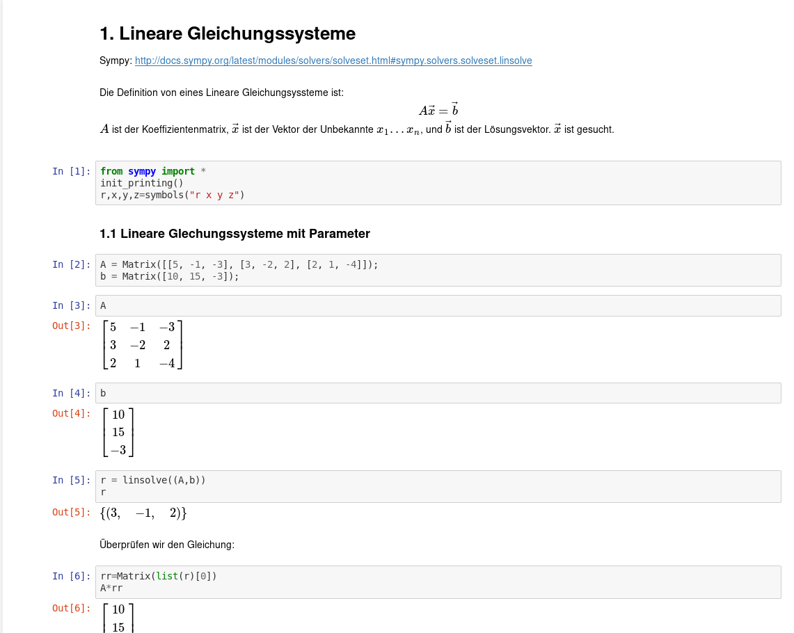
A Notebook is composed of “cells”, which are thingies in which code or rich text is run. One thing that I did not find intuitive with Jupyter is how all the variables are kept in memory until you restart the kernel. That is, if you have, say

r=linsolve((A,b))

in one cell,

print(r)

in the second, and

r=nonlinsolve((O,H))

in the next one, if you come back to the second cell, it will output the last thing it remembers for “r”, even if the value was set several cells below the one you are running now.

Another thing I had problems with (which also is not Jupyter’s problem) is the imports. That is, import * from math  meant that, for example, when I wanted to use sqrt()  it took math ‘s function with the same name, which is a numeric sqrt, not symbolic, and errored out (I’ll complain about Sympy’s errors a bit later).

Jupyter supports Markdown and LaTeX (which I recently learned is pronounced [lay-tech]) which allowed me to insert nice formulas and pictures:

Jupyter allows exporting to html and pdf, among other formats. I was pleasantly surprised that, for example, the HTML export left my plot animation animated. And in general, it has a really nice infrastructure around it, I mentioned the Notebook-vim  plugin above (and I’m not surprised a way to control Jupyter from vim also exists), but there are many more (again, open source is nice). A second program I used heavily was nbmerge, which allowed me to merge multiple notebooks into a big one (and creating a mess with the variable names and imports…). It’s used predictably:

nbmerge 1. 1.\ Lineare\ Gleichungsyssteme.ipynb NichtLin.ipynb 3.\ Newton-Int\ and\ Spline-int.ipynb 4.\ Standort.ipynb > merged.ipynb

Jupyter is awesome. I used it later for my own project about analyzing messages in a big groupchat (I’ll probably post a write-up here when I finish it) and will probably use it for any other projects requiring quick and easy inline graphs/plots/visualizations.

2. Sympy

Now playing: Alphaville – Big in Japan

Sympy is a Python library for symbolic mathematics (that is, dealing with mathematical expressions, transforming them, intergrating, substituting variables etc., as opposed to working just with numbers).

I used it heavily, it allowed (or was supposed to allow) to do everything that I needed. I found it a very simple and pleasant library to work with. For a very basic example, refer to any of the screenshots above. It was really nice working on formulas directly. Say, here:

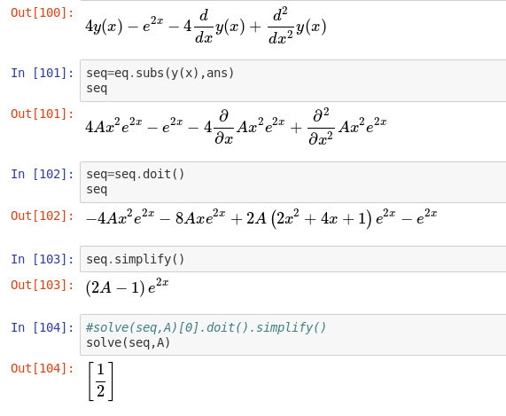
In [100], we have a differential equation. In [101], we substitute y(x)  as ans , which contains one of the solutions, and get another equation. Then seq.doit()  computes the differentials. We get a long equation which we .simplify() , and get the small equation [103]. We solve it for A and get 1/2. Isn’t this nice?

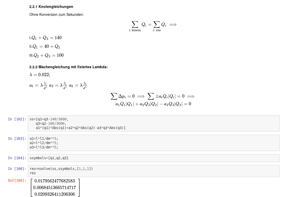
Or here, when I needed three very similar and very long formulas for the, um, flow rate in a system of three tubes:

Re1=(4*Abs(q1))/(pi*dm*v);

ins1=(
    (2.51/
     (Re1*sqrt(la1))
    ) +
    k/(3.71*dm)
)
    
zg1 = (1/sqrt(la1))+2*log(ins1,10);

zg2=zg1.subs(la1,la2);
zg2=zg2.subs(q1,q2);

zg3=zg1.subs(la1,la3);
zg3=zg3.subs(q1,q3);

I created the second two formulas by substituting the constanst lambda1 and Q1 for lambda2,3 and Q2,3 instead of needing to copypaste the whole thing (and make errors in the process). And I could split the formula to multiple lines and brackets, since it all in one line would have been hellish.

What I found really not helpful were the error messages, which could be charitably described as “not intuitive”.

For example. It’s hard enough when you don’t know the math. It’s harder when you don’t know neither the math you are trying to use nor the software. Especially if it gives you some weird error message 17 functions deep. Like using y  instead of y(x) , even after you’ve told Sympy that y is a function from x, helfully returns:

TypeError: as_base_exp() missing 1 required positional argument: 'self'

But life gets really interesting when you know that there’s a third place where errors could happen: the software itself. Even if you do something that makes sense matematically, you’ve written it correctly and used the right functions, it fails. And gives some really obscure error, exactly the same kind as when you make an error. For example, here. At some point Sympy stopped computing Laplace transforms of piecewise functions. Everyone agreed that it doesn’t do this anymore and it’s a problem. Then everyone happily forgot about it. Nothing in the documentation about that.

Or this. This discussion was hard to find. In my case I was trying to plot splines. Apparently Sympy doesn’t play well with undefined logarithms, and by extension with things that might want to compute one of them. In the linked discussion, the solution is to plot not from x=0 , but from x=-1  (“— Doctor, my hand hurts when I move it like this. — Well then don’t move it like this!”). In my case it didn’t help since there was a log(0)  somewhere deep down. … and you wonder if it’s your faulty math, your faulty transcription (“could it be another y/y(x) thingy?”), or Sympy. Also apparently the Sympy plotter just can’t plot a series of points, just functions. At the end of the day, I decided to use Matplotlib, really happy about that.

Bugs in software are nothing new, and I really like open source in this respect — you can go as deep down the rabbit hole as you want, and read philosophical-theoretical-ideological discussions by the devs about what should be returned when log(0), but it doesn’t really help when you just want to graph a function. I am someone definitely used to weird errors you have to solve with or without the help of the Internet (wouldn’t be an Arch user otherwise), but still with Sympy it was a bit more frustrating than it usually is. BUT the 95% of what works works, and works wonderfully. And I’m not complaining — I technically should have the skills to help the project, and almost feel morally obligated to do so, but can not at this time. And Sympy seems to have a very lively developer community and Gitter channel. I still deeply respect everyone who donates their time to developing things they believe in. If I was working in a math field or was a more-than-once-in-my-life user of Sympy, I would seriously consider contributing.

(the feeling when you google your error and get ONE result, some guy who in 2008 had the same problem, no answers _— oh, denvercoder9, what did you find?)

As I reached Laplace transforms and Fourier transforms, I found I could not get them working in Sympy, and used Sage.

Regardless, Sympy is good, and I like much more than apparent from the paragraphs above. It can do most of what I needed it to do, and even though it was sometimes really frustrating (… the fact that I don’t know calculus, Python or Sympy well was definitely part of it), I’m still really glad that I used it instead of anything else.

3. Myplotlib/Pyplot

I did not finish my project in time for the exam partly because I discovered that Jupyter can do graphs. And spent definitely more time than would have been wise changing small details, and making the graphs perfect. Then I discovered that it can do ANIMATED PLOTS, and at that point I understood that there was no hope, no hope at all.

Now playing: Black – Wonderful Life

Matplotlib is basically the most typical way to plot stuff. I used Pyplot, which is part of Myplotlib.

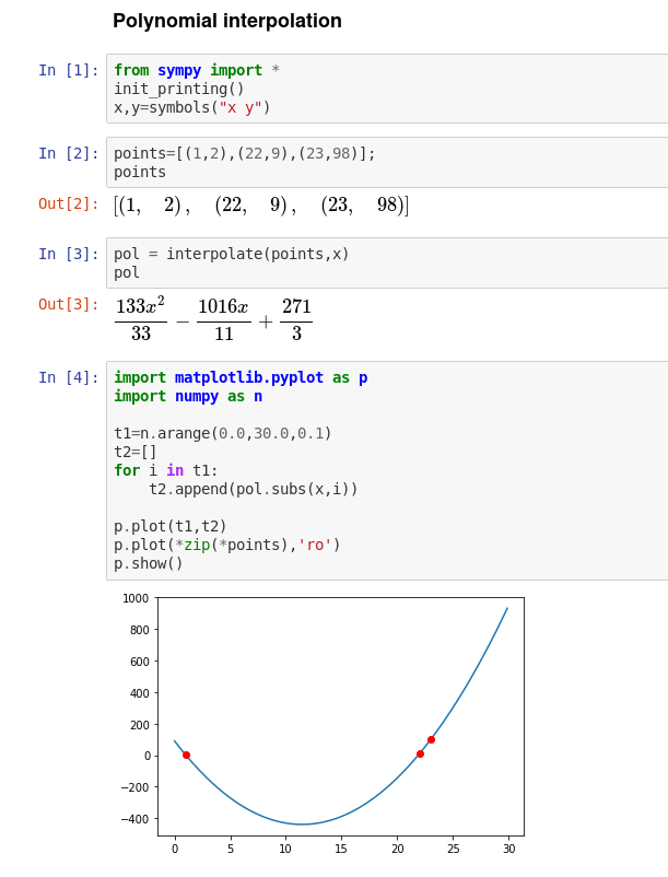
In the screenshot above you can see a typical use case. At the beginning, we generate a range of points from 0 to 30, with 0.1 distance inbetween (that is 300 points). Then we feed them to a function “pol”, where (via Sympy’s .subs ) we substitute the x with each of the generated x-points. Then we add t1 (the X-values) and t2 (Y-values) to the plot, since mpl wants the X and Y coords supplied separately. In the second-to-last line, we zip an array of three points ([[x,y],[xx,yy]]  to [[x,xx],[y,yy]] ), tell them to be red (‘r’) and points (‘o’) and also plot them. The last line shows our plot.

Another typical thing is a scatter plot.

p.grid();
p.scatter(x,y,w,norm(a),marker='o',linewidth='1',edgecolor='black')
p.scatter(xa,ya,c='yellow',marker='*',s=200,linewidth='1',edgecolor='black',alpha=0.9)

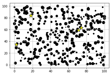
We create a grid. In the second line, we pass four main parameters — x, y, w as “size” and norm(a)  which is the colour, more about this part later. All of the other parameters should be self-explanatory. In the third line, same as above, except we pass the parameters explicitly, so the order doesn’t matter — color is yellow, and marker is “*”, which is a star. Then size etc. Last parameter is the opacity.

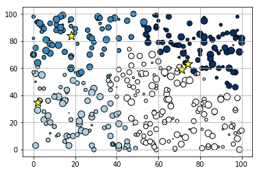
Colors in mpl are interesting. The function norm() was defined the following way, a bit above in the code: norm=colors.Normalize(vmin=0, vmax=nOfAP);  and it basically translates any number from 0 to nOfAP into a float in the 0..1 range. (See Colormap Normalization). Then Matplotlib takes this number from 0 to 1 and translates it into a color from a colormap. The link contains the colormaps mpl has available, highly suggest visiting it.

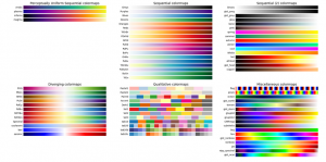
Also different colormaps have different use cases, and the theory behind that is very interesting. Some colormaps perform worse than others when the image gets printed in grayscale, for example. Here is a nice link on topic, the post also has links to other interesting places. The whole luminance thing was not obvious to me, I love learning about such things. Also see Ten simple rules for better figures.

Animating plots is a whole new matter. Below, you see the animated steps of my implementation of the Weiszfeld algorithm, where the airports (yellow stars) get positioned in the geometric median (red hexagons) at each iteration. Not much but I like it somehow.

Animations are created simply enough.

def update(i): // Gets run at every frame
    global universe; // Where all data from all steps of the algorithm is saved
    ax.clear() // Clear last frame

    scatter=ax.scatter(universe[i][0][0],universe[i][0][1],universe[i][0][2],norm(universe[i][0][3]),marker='o',cmap='Blues',linewidth='1',edgecolor='black') // points
    scatter=ax.scatter(universe[i][2][0],universe[i][2][1],c='yellow',marker='*',s=250,linewidth='1',edgecolor='black') // Stars
    scatter=ax.scatter(universe[i][1][0],universe[i][1][1],c='xkcd:hot pink',marker='H',s=150,linewidth='1',edgecolor='black') // Hexagons
    scatter=ax.text(5, -10, 'Step '+str(i), style='italic') // Step indicator (bottom row)
    print("Out of",len(universe),", we're at ",end='') // Show progress during the creation of the animation
    print(i,end=''); // without going to a newline every time
    return scatter;

anim = FuncAnimation(fig, update, interval=500,frames=len(universe)) // big interval; and as many frames as there were steps in the algorith before it stopped
plt.show()
from IPython.display import HTML,Image
rc('animation', html='html5') // animation as HTML5
anim // output animation

The point of this post is not to make a tutorial out of it, more like “Hey, this exists, I liked it, here’s what I found especially interesting”, and I guess it’s mission completed.

As usual, thank for reading, over and out.

(Y)